3. Correcting Bias in Ranking Data

library(rankingQ)
data(identity)

library(dplyr)
library(ggplot2)
library(tidyr)

Estimating the Proportion of Random Responses

In the identity dataset, given anc_correct_identity, the raw proportion of those who have correctly or incorrectly answered the anchor question is as follows:

round(prop.table(table(identity$anc_correct_identity)) * 100, digits = 1)

## 
##    0    1 
## 30.3 69.7

The 69.7% seen here, however, is likely an upwardly biased estimate of the percentage of non-random responses, because we must account for respondents accidentally answering the question correctly. For an unbiased estimate of random responses, we use unbiased_correct_prop.

identity$random_identity <- case_when(
  identity$anc_correct_identity == 1 ~ 0,
  TRUE ~ 1
)

unbiased_correct_prop(
  sum(identity$random_identity == 0) / sum(!is.na(identity$random_identity)),
  J = 4
)

## [1] 0.6836776

The revised estimate of non-random responses is 68.4%. That is to say, roughly 31.6% of the respondents are randomly responding.

Direct Bias Correction via `imprr_direct`

rankingQ has two primary functions to perform bias correction. First, imprr_direct improves ranking data by applying direct bias correction to several classes of quantities of interest.

To apply the bias correction, we specify our dataset (data), the number of items (J), the prefix of column names that contain J items for the target ranking questions, and the prefix of column names for the anchor ranking questions. When survey weights are available, they can be included by specifying weight in the function.

## app_identity_1 indicates marginal rank for party
## app_identity_2 indicates marginal rank for religion
## app_identity_3 indicates marginal rank for gender
## app_identity_4 indicates marginal rank for race

# Perform bias correction
out_direct <- imprr_direct(
  data = identity,
  ## Not strictly necessary if app_identity, the input for `main_q`,
  ## is specified. In that case, will look for J if unspecified
  J = 4,
  ## automatically looks for
  ## app_identity_1, app_identity_2, app_identity_3, app_identity_4
  main_q = "app_identity",
  anc_correct = "anc_correct_identity",
  # setting to 10 only for our vignette
  n_bootstrap = 10
)

## No weight column supplied; using equal weights for all observations.

By default, imprr_direct assumes that the target population is a set of non-random respondents. When researchers wish to study the entire population as a target group, additional arguments must be specified, including population and assumption. For example, the uniform preference assumption can be specified as follows:

# Bias correction for the entire population with the uniform assumption

out_direct_uniform <- imprr_direct(
  data = identity,
  J = 4,
  main_q = "app_identity",
  anc_correct = "anc_correct_identity",
  population = "all",
  assumption = "uniform",
  n_bootstrap = 10
)

## population = 'all' with assumption = 'uniform' implies no correction; ignoring anc_correct and p_random.

## No weight column supplied; using equal weights for all observations.

Similarly, the contaminated sampling assumption can be specified as follows:

# Bias correction for the entire population with contaminated sampling

out_direct_contaminated <- imprr_direct(
  data = identity,
  J = 4,
  main_q = "app_identity",
  anc_correct = "anc_correct_identity",
  population = "all",
  assumption = "contaminated",
  n_bootstrap = 10
)

## No weight column supplied; using equal weights for all observations.

Results: Estimated Proportion of Random Responses

The first output of imprr_direct is the estimated proportion of random responses. The vector est_p_random returns the estimated proportion along with the lower and upper ends of its corresponding 95% confidence interval.

# Estimated proportion of random responses with a 95% CI
out_direct$est_p_random

##        mean     lower     upper
## 1 0.3158402 0.2875352 0.3451338

Results: Estimated Quantities of Interest

The other output is the bias-corrected estimates of four classes of ranking-based quantities, including

average ranks
pairwise ranking probabilities
top-k ranking probabilities
marginal ranking probabilities

The output tibble qoi stores the estimated quantities and their corresponding 95% CIs.

# View the results based on the quantity of interest
out_direct$results %>%
  filter(qoi == "average rank")

## # A tibble: 4 × 6
##   item           qoi          outcome              mean lower upper
##   <chr>          <chr>        <chr>               <dbl> <dbl> <dbl>
## 1 app_identity_1 average rank Avg: app_identity_1  3.27  3.21  3.30
## 2 app_identity_2 average rank Avg: app_identity_2  2.60  2.49  2.66
## 3 app_identity_3 average rank Avg: app_identity_3  1.66  1.61  1.74
## 4 app_identity_4 average rank Avg: app_identity_4  2.48  2.42  2.53

# View the results based on the item
out_direct$results %>%
  filter(item == "app_identity_1")

## # A tibble: 11 × 6
##    item           qoi              outcome               mean  lower  upper
##    <chr>          <chr>            <chr>                <dbl>  <dbl>  <dbl>
##  1 app_identity_1 average rank     Avg: app_identity_1 3.27   3.21   3.30  
##  2 app_identity_1 marginal ranking Ranked 1            0.0427 0.0309 0.0638
##  3 app_identity_1 marginal ranking Ranked 2            0.151  0.133  0.171 
##  4 app_identity_1 marginal ranking Ranked 3            0.304  0.289  0.336 
##  5 app_identity_1 marginal ranking Ranked 4            0.503  0.488  0.520 
##  6 app_identity_1 pairwise ranking v. app_identity_2   0.359  0.335  0.382 
##  7 app_identity_1 pairwise ranking v. app_identity_3   0.109  0.0807 0.143 
##  8 app_identity_1 pairwise ranking v. app_identity_4   0.266  0.257  0.287 
##  9 app_identity_1 top-k ranking    Top-1               0.0427 0.0309 0.0638
## 10 app_identity_1 top-k ranking    Top-2               0.194  0.172  0.213 
## 11 app_identity_1 top-k ranking    Top-3               0.497  0.480  0.512

For example, one can visualize the result for average ranks as follows:

# Plot the result
out_direct$results %>%
  mutate(
    item = factor(
      item,
      levels = paste0("app_identity_", seq(4)),
      labels = c("party", "religion", "gender", "race")
    )
  ) %>%
  plot_avg_ranking()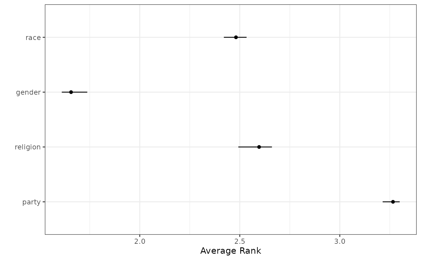

Weighting-Based Bias Correction via `imprr_weights`

The alternative method for bias correction is based on the idea of inverse-probability weighting (IPW). imprr_weights improves ranking data by computing bias correction weights, which can be used to correct for the bias in the IPW framework. The same arguments previously used can be used as follows:

Because imprr_weights enumerates the full permutation space, its computational cost grows quickly with J!. In practice, this method is best suited to small or moderate ranking questions; for larger J, imprr_direct or imprr_direct_rcpp will usually be much more practical.

# Perform bias correction
out_weights <- imprr_weights(
  data = identity,
  J = 4,
  main_q = "app_identity",
  anc_correct = "anc_correct_identity"
)

## No weight column supplied; using equal weights for all observations.

By default, imprr_weights assumes that the target population is a set of non-random respondents. When researchers wish to study the entire population as a target group, additional arguments must be specified, including population and assumption. For example, the uniform preference assumption can be specified as follows:

# Perform bias correction with the uniform preference assumption
out_weights_uniform <- imprr_weights(
  data = identity,
  J = 4,
  main_q = "app_identity",
  anc_correct = "anc_correct_identity",
  population = "all",
  assumption = "uniform"
)

## population = 'all' with assumption = 'uniform' implies no correction; ignoring anc_correct and p_random.

## No weight column supplied; using equal weights for all observations.

Similarly, the contaminated sampling assumption can be specified as follows:

# Perform bias correction with the uniform preference assumption
out_weights_contaminated <- imprr_weights(
  data = identity,
  J = 4,
  main_q = "app_identity",
  anc_correct = "anc_correct_identity",
  population = "all",
  assumption = "contaminated"
)

## No weight column supplied; using equal weights for all observations.

Results: Estimated Weights

The output of imprr_weights contains the set of weights for all possible ranking profiles with J items. For example, when J = 4, the set has {1234, 1243, ..., 4321} and each profile now has an estimated weight.

# View the estimated weights
out_weights$rankings %>%
  select(ranking, weights)

##    ranking   weights
## 1     1234 0.0000000
## 2     1243 0.0000000
## 3     1324 0.0000000
## 4     1342 0.0000000
## 5     1423 1.0158812
## 6     1432 0.4078355
## 7     2134 0.8582397
## 8     2143 0.8070574
## 9     2314 0.7456387
## 10    2341 0.0000000
## 11    2413 1.1316994
## 12    2431 0.5767371
## 13    3124 1.0238295
## 14    3142 0.5400194
## 15    3214 0.8251218
## 16    3241 0.0000000
## 17    3412 1.2733020
## 18    3421 1.0314721
## 19    4123 1.2628998
## 20    4132 1.1045545
## 21    4213 1.0388263
## 22    4231 0.4999637
## 23    4312 1.2711103
## 24    4321 1.0593130

Results: Estimated PMF with Bias Corrected Data

imprr_weights also returns the estimated probability mass function of all ranking profiles before and after bias correction.

# View the estimated corrected PMF
out_weights$rankings %>%
  select(ranking, prop_obs, prop_bc)

##    ranking    prop_obs     prop_bc
## 1     1234 0.012939002 0.000000000
## 2     1243 0.010166359 0.000000000
## 3     1324 0.012939002 0.000000000
## 4     1342 0.006469501 0.000000000
## 5     1423 0.046210721 0.046944603
## 6     1432 0.018484288 0.007538549
## 7     2134 0.033271719 0.028555111
## 8     2143 0.030499076 0.024614506
## 9     2314 0.027726433 0.020673901
## 10    2341 0.005545287 0.000000000
## 11    2413 0.064695009 0.073215306
## 12    2431 0.022181146 0.012792690
## 13    3124 0.047134935 0.048258138
## 14    3142 0.021256932 0.011479155
## 15    3214 0.031423290 0.025928041
## 16    3241 0.011090573 0.000000000
## 17    3412 0.126617375 0.161222159
## 18    3421 0.048059150 0.049571673
## 19    4123 0.118299445 0.149400343
## 20    4132 0.059149723 0.065334095
## 21    4213 0.048983364 0.050885208
## 22    4231 0.020332717 0.010165620
## 23    4312 0.124768946 0.158595089
## 24    4321 0.051756007 0.054825814

Estimated Weights with Original Data

identity_w <- out_weights$results
head(identity_w)

## # A tibble: 6 × 19
##   weights s_weight app_identity app_identity_1 app_identity_2 app_identity_3
##     <dbl>    <dbl> <chr>                 <dbl>          <dbl>          <dbl>
## 1    1.02    0.844 1423                      1              4              2
## 2    1.02    0.886 1423                      1              4              2
## 3    1.27    2.96  3412                      3              4              1
## 4    1.02    0.987 1423                      1              4              2
## 5    1.10    1.76  4132                      4              1              3
## 6    1.02    0.469 3124                      3              1              2
## # ℹ 13 more variables: app_identity_4 <dbl>, anc_identity <chr>,
## #   anc_identity_1 <dbl>, anc_identity_2 <dbl>, anc_identity_3 <dbl>,
## #   anc_identity_4 <dbl>, anc_correct_identity <dbl>,
## #   app_identity_recorded <chr>, anc_identity_recorded <chr>,
## #   app_identity_row_rnd <chr>, anc_identity_row_rnd <chr>,
## #   random_identity <dbl>, ranking <chr>

# save(identity_w, file = "data/identity_w.rda")

Yuki Atsusaka and Seo-young Silvia Kim