2. Correcting Bias in Ranking Data

Direct Bias Correction via `imprr_direct`

rankingQ has two primary functions to perform bias correction. First, imprr_direct improves ranking data by applying direct bias correction to several classes of quantities of interest.

To apply the bias correction, we specify our dataset (data), the number of items (J), the prefix of column names that contain J items for the target ranking questions, and the prefix of column names for the anchor ranking questions. When survey weights are available, they can be included by specifying weight in the function.

library(rankingQ)
library(dplyr)
library(ggplot2)
library(tidyr)

# Rename the items with a common prefix
identity <- identity %>%
  rename(
    app_identity_1 = app_party,
    app_identity_2 = app_religion,
    app_identity_3 = app_gender,
    app_identity_4 = app_race
  )

# Perform bias correction
out_direct <- imprr_direct(
  data = identity,
  J = 4,
  main_q = "app_identity",
  anc_correct = "anc_correct_identity"
)

Results: Estimated Proportion of Random Responses

The first output of imprr_direct is the estimated proportion of random responses. The vector est_p_random returns the estimated proportion along with the lower and upper ends of its corresponding 95% confidence interval.

# Estimated proportion of random responses with a 95% CI 
out_direct$est_p_random

##        mean     lower     upper
## 1 0.3153146 0.2864261 0.3481958

Results: Estimated Quantities of Interest

The other output is the bias-corrected estimates of four classes of ranking-based quantities, including

average ranks
pairwise ranking probabilities
top-k ranking probabilities
marginal ranking probabilities

The output tibble qoi stores the estimated quantities and their corresponding 95% CIs.

# View the results based on the quantity of interest
out_direct$qoi %>%
   filter(qoi == "average rank")

## # A tibble: 4 × 6
## # Groups:   item, qoi [4]
##   item           qoi          outcome              mean lower upper
##   <chr>          <chr>        <chr>               <dbl> <dbl> <dbl>
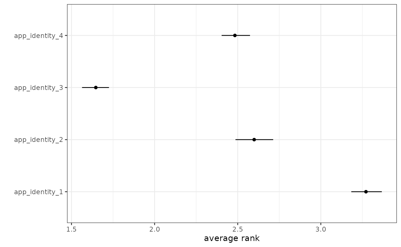
## 1 app_identity_1 average rank Avg: app_identity_1  3.27  3.18  3.37
## 2 app_identity_2 average rank Avg: app_identity_2  2.60  2.49  2.71
## 3 app_identity_3 average rank Avg: app_identity_3  1.65  1.56  1.73
## 4 app_identity_4 average rank Avg: app_identity_4  2.48  2.40  2.57

# View the results based on the item
out_direct$qoi %>%
  filter(item == "party")

## # A tibble: 0 × 6
## # Groups:   item, qoi [0]
## # ℹ 6 variables: item <chr>, qoi <chr>, outcome <chr>, mean <dbl>, lower <dbl>,
## #   upper <dbl>

For example, one can visualize the result for average ranks as follows:

# Plot the result
out_direct$qoi %>%
  filter(qoi == "average rank") %>%
  ggplot(aes(x = mean, y = item)) +
  geom_point() +
  geom_linerange(aes(xmin = lower, xmax = upper)) +
  theme_bw() +
  xlab("average rank") +
  ylab("")

Weighting-Based Bias Correction via `imprr_weight`

The alternative methods for bias correction is based on the idea of inverse-probability weighting. imprr_weight improves ranking data by computing bias correction weights, which can be used to correct for the bias in the inverse-probability weighting framework. The same arguments previously used can be used as follows:

# Perform bias correction
out_weights <- imprr_weights(
  data = identity,
  J = 4,
  main_q = "app_identity",
  anc_correct = "anc_correct_identity"
)

Results: Estimated Weights

The output of imprr_weights contains the set of weights for all possible ranking profiles with J items. For example, when J = 4, the set has {1234, 1243, ..., 4321} and each profile now has an estimated weight.

# View the estimated weights
out_weights$weights

##    ranking         w
## 1     1234 0.0000000
## 2     1243 0.0000000
## 3     1324 0.0000000
## 4     1342 0.0000000
## 5     1423 1.0158812
## 6     1432 0.4078355
## 7     2134 0.8582397
## 8     2143 0.8070574
## 9     2314 0.7456387
## 10    2341 0.0000000
## 11    2413 1.1316994
## 12    2431 0.5767371
## 13    3124 1.0238295
## 14    3142 0.5400194
## 15    3214 0.8251218
## 16    3241 0.0000000
## 17    3412 1.2733020
## 18    3421 1.0314721
## 19    4123 1.2628998
## 20    4132 1.1045545
## 21    4213 1.0388263
## 22    4231 0.4999637
## 23    4312 1.2711103
## 24    4321 1.0593130

Results: Estimated PMF with Raw Data and Bias Corrected Data

imprr_weight also returns the estimated probability mass function of all ranking profile before and after bias correction.

# View the estimated PMF with raw data and weighted data
out_weights$corrected_pmf %>%
  select(ranking, prop, prop_renormalized)

##    ranking          prop prop_renormalized
## 1     1234 -0.0003526508       0.000000000
## 2     1243 -0.0044081345       0.000000000
## 3     1324 -0.0003526508       0.000000000
## 4     1342 -0.0098154461       0.000000000
## 5     1423  0.0483131539       0.046944603
## 6     1432  0.0077583167       0.007538549
## 7     2134  0.0293875632       0.028555111
## 8     2143  0.0253320795       0.024614506
## 9     2314  0.0212765957       0.020673901
## 10    2341 -0.0111672740       0.000000000
## 11    2413  0.0753497120       0.073215306
## 12    2431  0.0131656283       0.012792690
## 13    3124  0.0496649818       0.048258138
## 14    3142  0.0118138004       0.011479155
## 15    3214  0.0266839074       0.025928041
## 16    3241 -0.0030563066       0.000000000
## 17    3412  0.1659221817       0.161222159
## 18    3421  0.0510168097       0.049571673
## 19    4123  0.1537557306       0.149400343
## 20    4132  0.0672387446       0.065334095
## 21    4213  0.0523686376       0.050885208
## 22    4231  0.0104619725       0.010165620
## 23    4312  0.1632185259       0.158595089
## 24    4321  0.0564241213       0.054825814

Merge Estimated Weights with Original Data

# Turn the results into a tibble
tibble_w <- out_weights$weights %>% tibble()

# Merge the weights back to the original data
identity_w <- identity %>%
  unite(ranking, starts_with("app_identity"), sep = "", remove = FALSE) %>%
  left_join(tibble_w, by = "ranking") %>%
  select(w, everything()) %>%
  rename(
    party = app_identity_1,
    religion = app_identity_2,
    gender = app_identity_3,
    race = app_identity_4
  )
head(identity_w)

## # A tibble: 6 × 12
##       w ranking party religion gender  race anc_house anc_neighborhood anc_city
##   <dbl> <chr>   <dbl>    <dbl>  <dbl> <dbl>     <dbl>            <dbl>    <dbl>
## 1  1.02 1423        1        4      2     3         1                2        3
## 2  1.02 1423        1        4      2     3         1                2        3
## 3  1.27 3412        3        4      1     2         1                2        3
## 4  1.02 1423        1        4      2     3         1                2        3
## 5  1.10 4132        4        1      3     2         1                3        2
## 6  1.02 3124        3        1      2     4         1                2        3
## # ℹ 3 more variables: anc_state <dbl>, anc_correct_identity <dbl>,
## #   s_weight <dbl>

Yuki Atsusaka and Seo-young Silvia Kim

Direct Bias Correction via imprr_direct